A brief analysis of gender distribution in visual representations of everyday life in North Korea using facial recognition algorithms and transfer learning applied to convolutional neural networks.

1. The Data

A couple months ago, I was invited to participate in a workshop on North Korean posters organized by Prof. Koen de Ceuster at Leiden University in the Netherlands. The posters came from the private collection of Willem van der Bijl, a Utrecht-based stamp dealer, who had been purchasing North Korean posters regularly for over a decade. Prof. de Ceuster had arranged to get the posters digitalized and they are now available as part of Leiden University’s Digital Collections. Access to the collection currently still requires an account, but this might change in the future.

 

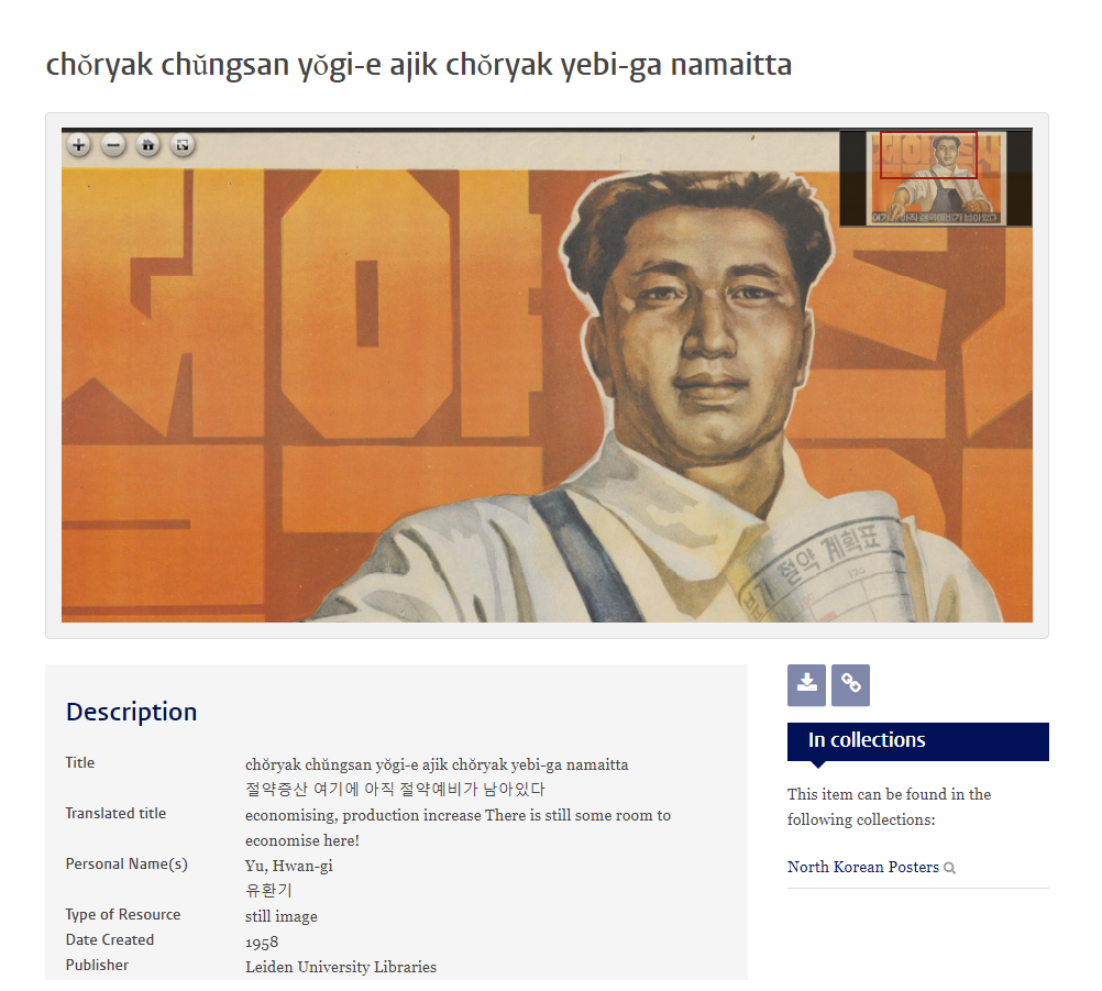
Each poster in the collection has been enriched with metadata such as its title, the name of the artist and date of production (if available), the main themes, a brief description of the poster’s content and various technical details. The posters can be viewed directly on the website through a viewer plug-in or downloaded through the provided links. While the viewer lets us zoom to a high-resolution version of each poster, the only version available for download is fairly small and low-resolution. With a small scraping script, I’ve made a local copy of the posters and stored the metadata in a collection on a MongoDB database. Given this great amount of both textual and visual data spanning over the (almost) entire history of the DPRK, I thought it could be fun to do a bit of data mining and try to extract some statistics to get a general idea of the imagery that these posters circulated.

2. Face Detection and Gender Classification

The posters’ metadata contains topical tags that tells us whether the poster is about industry, agriculture, sports… There is however much less information about who, if anyone, actually is in the posters. Some posters have an extra entry in their database with a detail description of their content, but they are relatively few in numbers. We can, however, use some computer vision algorithm to detect people in posters and classify them by gender. This, in turn, would give us a sense of how social activities are gendered in the DPRK.

Let’s start with some code. Face detection is a classic computer vision problem, which aims at determining whether there are any (human) faces within an image. Fortunately, for 2D static images, algorithms are now well-developed and widely available, with state-of-the art methods performing with roughly 80% accuracy overall and close to, or over, 90% for large faces. For those interested in the history of facial detection and recognition, a fascinating book by Prof. Kelly Gates offers an investigation of the cultural practices, social constructs and technocratic illusions behind the development of this technology since the 1960’s.

Since available face detection algorithms are trained on real-life pictures rather than drawings, their might not perform as well on our dataset. However, because North Korean art is heir to socialist realism, characters in the posters are depicted very realistically and their facial topology closely resembles that of a real-life human face. We are also mostly interested in the central figures of the poster, so the weaker detection rate on smaller, background faces is actually more of a noise filter for our task. Finally, the fact that the posters are artistic depictions also gives us an advantage over usual photographic datasets. One of the main challenges to face detection algorithm is pose, with awkward angles having a very negative impact on accuracy. Because the characters’ poses in the posters are all aesthetically staged and predominantly forward facing, their faces should be easier to recognize.

To perform the face detection we’ll use the face_recognition Python package. The package itself requires the Boost C++ library and dlib for Python, both of which can prove complex to install (instructions here and here). Because both size and resolution affect the detection of faces, the pictures will be rescaled by a factor of 2.5, which I found improved both accuracy and recall. Once a face has been found, we’ll isolate the region of the picture where it was detected and perform face alignment on it using the imutils package. Face alignment is the operation of detecting the main keypoints of a face (nose, eye, jawline…) then applying the necessary affine transforms (scaling, rotation, translation…) so that the keypoints are projected to a canonical position. This is a bit like data normalization, making sure all of our data is on a similar scale and position. Finally, the faces will be saved to a separate folder:

from imutils.face_utils import FaceAligner
from dlib import rectangle
import face_recognition
import imutils
import dlib
import cv2
import os

def resize(img):
    resized = cv2.resize(img, (0,0), fx=2.5, fy=2.5)
    return resized

detector = dlib.get_frontal_face_detector()
predictor = dlib.shape_predictor("shape_predictor_68_face_landmarks.dat") #path to the dlib model shape_predictor_68_face_landmarks.dat
fa = FaceAligner(predictor, desiredFaceWidth=224)

images = os.listdir('Posters')
for i, index in enumerate(images):
    print(index, ':', i, '/', len(images))
    image_path = 'Posters\\' + index + '\\' + index + '.jpg'
    img = cv2.imread(image_path)
    img = resize(img)
    gray = cv2.cvtColor(img, cv2.COLOR_BGR2GRAY)
    face_locations = face_recognition.face_locations(img, number_of_times_to_upsample=0)
    
    for j, face_location in enumerate(face_locations):
        
        top, right, bottom, left = face_location
        dlib_rect = rectangle(left, top, right, bottom) #convert to dlib rect object
        faceOrig = imutils.resize(img[top:bottom, left:right], width=224)
        faceAligned = fa.align(img, gray, dlib_rect)        
        cv2.imwrite('faces/' + index + '_' + str(j) + '.jpg', faceAligned)

This gives us a total of 1,525 faces, which we will now need to classify per gender.  There are no out-of-the box gender detection libraries and the open source classifiers that were trained on photos of real humans performed only slightly better than random on the posters’ faces, with roughly 60% accuracy. Since there aren’t that many images we could of course do the classification by hand, which would give much better accuracy. But this would be tedious and repetitive, and we would have to do it again every time new posters are added to the collection. Since we’re not looking for perfect accuracy, we can try to use machine learning instead to build a sufficiently robust classifier that we could use again in the future.

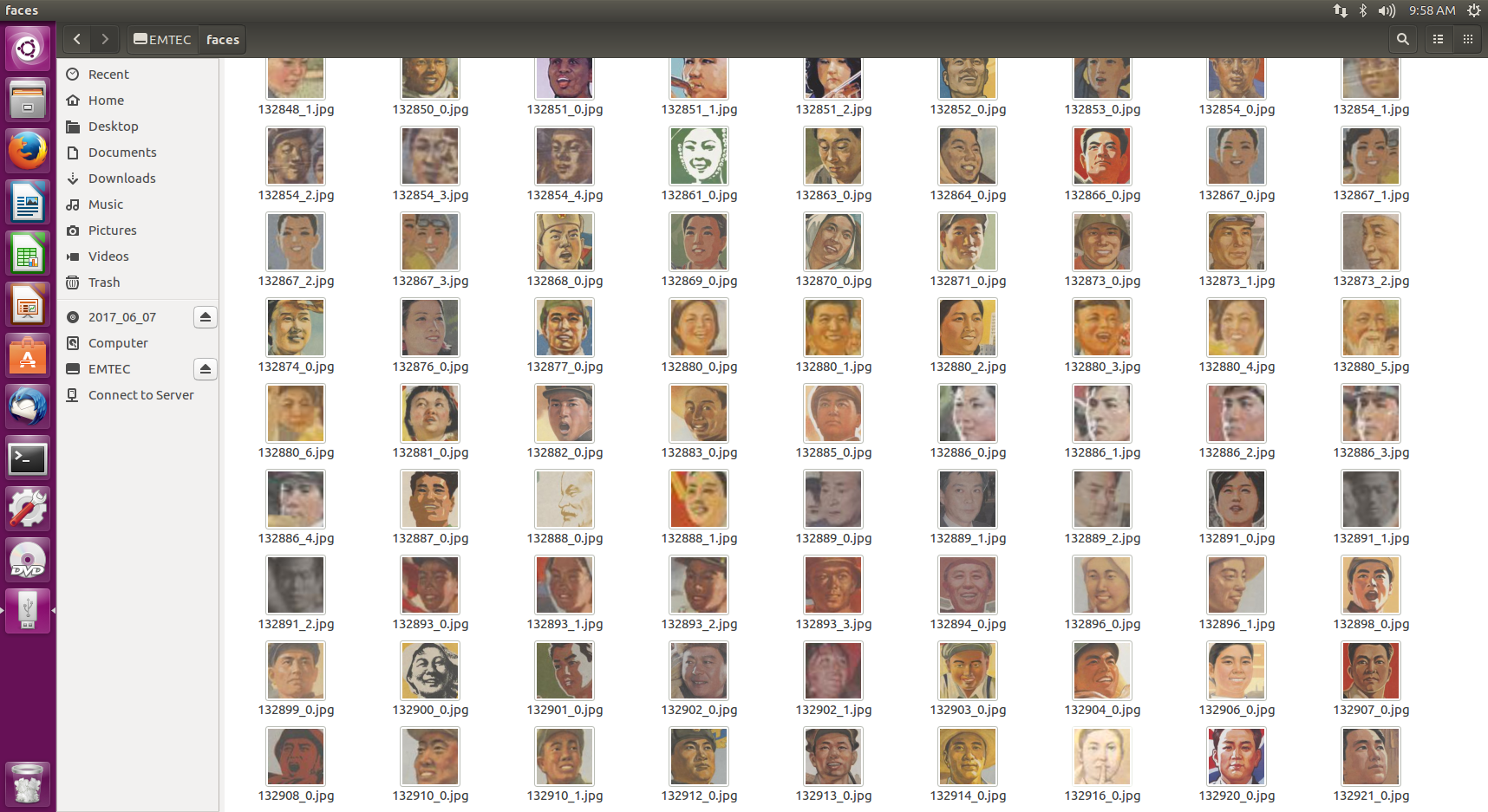
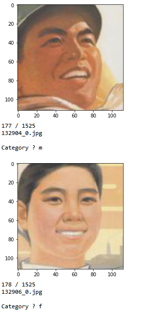
To do so, we will still need to do *some* classifying by hand, in order to construct a dataset on which we can train and test our algorithm. A few lines of Python can make this process significantly easier by displaying each face in the console, asking us to identify the gender, then copy the file to a sorted directory structure. We’ll have two directories, one for training and one for testing, each of which will contain a ‘male’ and ‘female’ folder. When we identify the gender of a face, the script automatically copies the source image to the train directory in 75% of the time and to the test directory 25% of the time. Finally, there is also an option to discard an image when we encounter a false positive from the earlier face detection step.

import cv2
import os
import matplotlib.pyplot as plt

images = os.listdir('faces')
def smaller(img):
    resized = cv2.resize(img, (0,0), fx=1/2, fy=1/2)
    return resized

plt.axis('off')

for index, image in enumerate(images):
    img = cv2.imread('faces/' + image)
    img = smaller(img)
    plt.imshow(cv2.cvtColor((img), cv2.COLOR_BGR2RGB))
    plt.show(block=False)
    category = ''
    while category not in ['m', 'f', 'o']:
        print(index, '/', len(images))
        print(image)
        category = input('Category ? ')
        
    if index % 4 == 0:
        path = 'data7/test'
    else:
        path = 'data7/train'
        
    if category == 'm':
        cv2.imwrite(path + '/male/' + image, img)
    elif category == 'f':
        cv2.imwrite(path + '/female/' + image, img)
    elif category == 'o':
        cv2.imwrite('data7/other/' + image, img)

After sorting about 300 pictures, or roughly 1/5th of the whole dataset we end up with 220 training faces (140 male / 80 female) and 70 testing faces (30 female / 40 male):

Now that we have the data, we need to pick an algorithm to train. For an image classification task such as this one, a convolutional neural network (CNN) would normally be the ideal candidate but 200 and something picture is way too little data to effectively train a CNN from scratch. Without, millions of samples at our disposal, it seems like we may need to find a non deep-learning solution. We could try to use methods such as Eigenfaces or Fisherfaces for feature extraction and pass the result to a non-deep-learning binary classifier. A simple attempt using fisherfaces  (code available on GitHub) gave slightly over 80% accuracy and recall, which certainly isn’t bad but is not great either.

A better option which would allow us to leverage the performance of neural networks without the need for humongous training data is Transfer Learning. We can attempt to use the “knowledge” gained by another deep-learning model trained for a fairly similar task over a much larger amount of data. For a CNN already trained to perform an image classification task, this means we can “cut the head” of the model by removing the final fully-connected layers performing the classification and re-use the output of the other layers to feed into our own classifier. We would therefore only keep the convolutional layers and use them as a feature extractor. Because the model has been trained on similar data, but on a much larger scale, it has had the chance to learn a wide range of features that will also be relevant to our classification task and which we would never be able to learn from a dataset made up of a few dozen pictures.

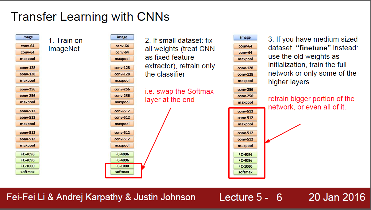
A good candidate for transfer learning for our model would be the VGG-Face CNN, a deep architecture based model trained for a face identification task on 2.6 million pictures. The Python version of the model is available as part of the deep learning library Keras, which will make our work much easier.

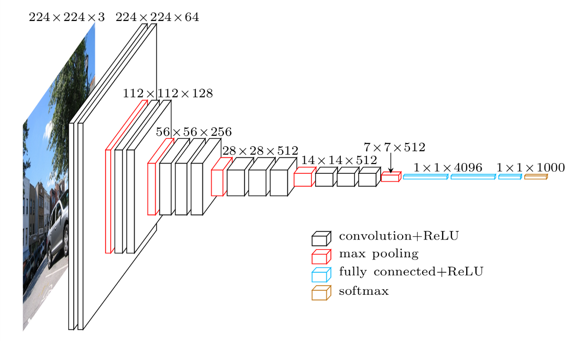
We will reuse the convolutional layers of VGG-Face, then add our own classifier with two fully connected layers and a sigmoid activation layer (as we will be performing a binary classification task – gender is not overly fluid in the DPRK) and train the model over 100 epochs. Note the use of a Generator class: even if our dataset is fairly small, the images we input are large enough (224×224, RGB) that we would not want to try and load them all at the same time in memory. The generator allows us to load the dataset in separate parts and send it on the fly as an input to our model. This is somewhat similar to Keras’ ImageDataGenerator feature, but having one’s own class gives a bit more flexibility:

import os
import numpy as np
from keras.models import Sequential
from keras.layers import Dense, Dropout
from keras_vggface.vggface import VGGFace
from inspect import getsourcefile
from os.path import abspath
from generator import Generator

path = os.path.dirname(abspath(getsourcefile(lambda:0)))

categories = os.listdir(os.path.join(path, 'data7/test'))
y_train = []
X_train = []
y_test = []
X_test = []
batch_size = 10
print('Getting samples')

for i, category in enumerate(categories):
    print(category)
    samples = os.listdir(os.path.join(path, 'data7/test', category))
    for sample in samples:
        X_test.append(os.path.join(path, 'data7/test', category, sample))
        y_test.append(i)

for i, category in enumerate(categories):
    print(category)
    samples = os.listdir(os.path.join(path, 'data7/train', category))
    for sample in samples:
        X_train.append(os.path.join(path, 'data7/train', category, sample))
        y_train.append(i)


training_generator = Generator(width = 224, height = 224, channels = 3, batch_size = batch_size).generate(X_train, y_train, return_labels = False, shuffle = False)
testing_generator = Generator(width = 224, height = 224, channels = 3, batch_size = batch_size).generate(X_test, y_test, return_labels = False, shuffle = False)

def save_features():
    model = VGGFace(include_top=False, input_shape=(224, 224, 3), weights='vggface', pooling = 'avg')              
    bottleneck_features_train = model.predict_generator(training_generator, len(X_train) // batch_size)
    np.save(open('bottleneck_features_train.npy', 'wb'), bottleneck_features_train)
    
    bottleneck_features_test = model.predict_generator(testing_generator, len(X_test) // batch_size)
    np.save(open('bottleneck_features_testing.npy', 'wb'), bottleneck_features_test)


def create_model():
    train_data = np.load(open('bottleneck_features_train.npy', 'rb'))
    train_labels = np.array([0] * 80 + [1] * 140)
    train_labels = train_labels[:len(train_labels) - (len(train_labels) % batch_size)]
    
    validation_data = np.load(open('bottleneck_features_testing.npy', 'rb'))
    validation_labels = np.array([0] * 30 + [1] * 40)
    validation_labels = validation_labels[:len(validation_labels) - (len(validation_labels) % batch_size)]
    
    model = Sequential()
    model.add(Dense(256, activation='relu', input_shape=train_data.shape[1:]))
    model.add(Dropout(0.5))
    model.add(Dense(64, activation='relu'))
    model.add(Dropout(0.5))
    model.add(Dense(1, activation='sigmoid'))

    model.compile(optimizer='rmsprop',
                  loss='binary_crossentropy', metrics=['accuracy'])
    
    model.fit(train_data, train_labels,
              epochs=100,
              batch_size=batch_size,
              validation_data=(validation_data, validation_labels))

    score = model.evaluate(validation_data, validation_labels)
    print('Test loss:', score[0])
    print('Test accuracy:', score[1])
    print("Baseline Error: %.2f%%" % (100-score[1]*100))

And the results after calling save_features() and create_model():

Epoch 95/100
220/220 [==============================] – 0s – loss: 0.0091 – acc: 0.9955 – val_loss: 1.7121 – val_acc: 0.8714
Epoch 96/100
220/220 [==============================] – 0s – loss: 0.0328 – acc: 0.9909 – val_loss: 0.7962 – val_acc: 0.9143
Epoch 97/100
220/220 [==============================] – 0s – loss: 0.1059 – acc: 0.9727 – val_loss: 0.8883 – val_acc: 0.9000
Epoch 98/100
220/220 [==============================] – 0s – loss: 0.0445 – acc: 0.9864 – val_loss: 0.7507 – val_acc: 0.9143
Epoch 99/100
220/220 [==============================] – 0s – loss: 0.0226 – acc: 0.9864 – val_loss: 0.8338 – val_acc: 0.9143
Epoch 100/100
220/220 [==============================] – 0s – loss: 0.0279 – acc: 0.9909 – val_loss: 0.8331 – val_acc: 0.9429
32/70 [============>……………..] – ETA: 0sTest loss: 0.833102767808
Test accuracy: 0.942857142857
Baseline Error: 5.71%

We might be able to make slight improvements by fiddling with the final classifier or using data augmentation techniques to artificially inflate the dataset, but the results are already satisfactory given such limited training data. We can now train the model on both the training and test dataset and use it to label the whole collection of faces, the results are as accurate as we expected:

3. Some Charts and Numbers

Now that the faces have been extracted and labelled, we can start to crunch some numbers. Let’s start with some general statistics:

Men are almost twice as prevalent as women on the posters and are also much more likely to appear alone or among members of their own gender. This unbalanced distribution has been fairly constant throughout the country’s history, despite an improvement in the 2000’s :

An interesting feature of the above chart is the dent of the 1990’s, suggesting that posters from this period are underrepresented in the collection. This might be explained by the scarcity of paper during the period of the North Korean famine. This could indicate that the famine had a strong impact on the state’s agitprop efforts, resulting in the number of posters dropping by more than half over the decade. Or this could be due to procurement issues on the part of the collector.

Because the poster’s metadata includes tags, we can also try to analyze the gender distribution for some of them. First let’s list the most common keywords:

And now the gender distribution:

While the keyword “economy” is a bit too large to be of use, the next most common keyword “agriculture” has an interesting pattern since the gender imbalance is reversed and we have more female characters than male. Another agriculture related keyword, “rice planting”, shows the same reversed ratio. On the other hand if we look at keywords related to the secondary sector, such as “industry”, “mining” or “construction” we see the opposite situation, with men being much more represented than in other categories.

This is more than just a reflection of employment demographics : especially in the agricultural sector, class appartenance is much more a matter of households than of individuals. Rather, the association of agricultural labor with women and industrial labor with men draws upon a long iconographic tradition in the socialist world. Besides agriculture, the other area were women are overrepresented in comparison to men is home management (“consumer goods”, “savings”…) suggesting that old patriarchal traditions die hard, even in revolutionary North Korea.

Military matters (“defense”, “army”, “songun”) and more generally politics (“ideology”, “anti-americanism”, “supreme people’s assembly”) display a stronger than average imbalance in favor of men and reflect a very real demographic distribution as more than 80% of the North Korean Supreme People’s Assembly is male (almost exactly the same as in South Korea’s parliament).

---

I mentioned earlier that some of the posters included a brief description of their content in the metadata. To supplement the statistics we’ve extracted using the visual data, we can try to mine this extra source of information to see if we can uncover some similar trends. To do so we can iterate over the whole metadata collection, everytime the word ‘male’ or ‘female’ shows up, we’ll capture the following nouns which should describe the occupation of the male or female in question. The task is trivial, using spaCy for the tokenization and pos-tagging, the following function will do the job, desc being the poster’s description, gender a string containing either ‘male’ or ‘female’ and gender_dict the defaultdict variable (set with values equal to 0) where we’ll store our counts:

def extract_info(desc, gender, gender_dict):
    doc = nlp(desc)
    indices = [i for i, x in enumerate(doc) if x.lemma_ == gender]
    for index in indices:
        s = ''
        i = index + 1
        gender_dict['total'] += 1
        while ((i < len(doc)) and
               (doc[i].pos_ in filters)):
            s += doc[i].lemma_ + ' '
            print('s', s)
            i += 1
            
        if s != '':  
            gender_dict[s.strip()] += 1

Which gives us the following results for males:

and for females:

We can notice again the relative predominance of representation of female agricultural workers and, inversely, that of male characters in industry related occupations. Textile and light industry posters have female characters but no male ones hinting at what the gender repartition may be within this particular economic sector. Finally, it is worth noting that for 77 description mentioning the word “female” there are only 66 mentioning the word “male”, most likely because when the central figure of a poster is male, the gender characteristics tend to be omitted from the description. To sum up, if we group the minor categories into larger ones, we can sum up the data mined from textual descriptions with the following graph:

4. Methodological Implications and Limitations

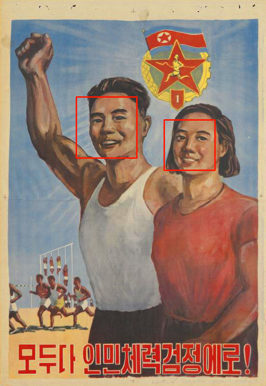
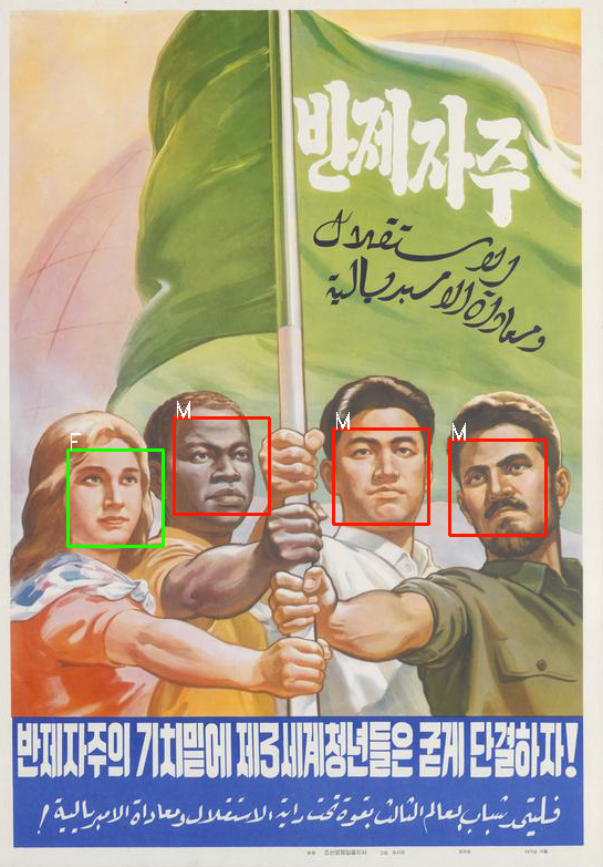
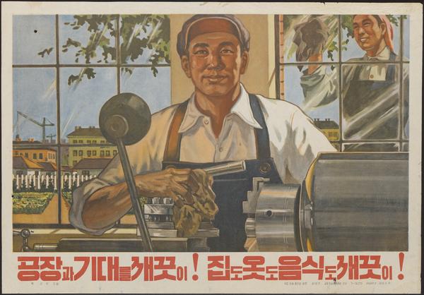
The quantification of certain aspects of visual or textual data as well as the compilation of statistics is clearly no substitute for a detailed qualitative analysis.  The current approach does not account for variations within representations of a similar category either: there might a wide variety of different female agricultural workers that we can’t account for, or similarly there might be differences in the way male and female workers are portrayed, as the poster below demonstrates:

However, using data and statistics allows one to make more robust assertions when dealing with issues of representations. A still common approach in fields such as literature and cultural studies is to take a limited corpus of texts or visuals and analyze them as symptomatic of a more general phenomenon. A few representations are taken as representative of all representations. But the truth of this postulate, the degree to which an argument developed on the analysis of a few limited example might actually generalize or “scale” to reality is in fine guaranteed by the authority of the writer or the brilliance of his analysis rather than by a large body of converging evidence.

Extracting information from large amount of data can not only strengthen an argument, but it can also help to perform quick hypothesis testing before engaging in further research. Simple data processing techniques and data visualizations, such as the ones employed here, allow one to rapidly detect points of interests and evacuate hypothesis who do not appeared to be supported by the data.

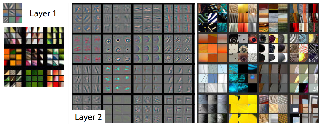
On the other hand, quantification is not necessarily a guarantee of objectivity : the algorithms employed all have limitations that can pile up and introduce some significant biases in the end-result. The approach developed in this article was more on the POC level, and an actual academic application would need better metrics and further explanations to better explain the limitations and biases potentially introduced by the model. Another limitation is the “black-box” aspect of more complex algorithms such as CNNs : while it’s possible to visualize and get an understanding of some of the features used by the network, they are hardly self-explanatory and in some cases, can be too abstract to be properly explained. The question then would be whether reproducibility and a model’s design are enough to warrant scientific veracity or whether a deeper explanation of what the model did and how it extracted its features should also be part of the analysis.