Designing a pre-processing method to improve OCR results using Python and OpenCV for old North Korean print material. Creating a simple character segmentation algorithm using contouring and simple heuristics. 

2. Preprocessing the Data: Character Segmentation

Following up on the previous post, we now have a working scraper that will let us download any RG-242 document from the Korean National Library’s website. We can use this to start working on an OCR solution for the files we have downloaded. For the rest of this post, we will work on the March 1949 issue of the 영화 예술 (Cinema Art) magazine, available here. There is no particular reason for this choice, but in terms of paper quality, typography, design and preservation, the magazine is quite representative of the other types of periodicals that are available in RG-242. The paper the magazine was printed on was not bleached and has darkened with age. It has a rough, grainy texture which will add some significant noise for an OCR task. The paper is also very thin and the characters printed on the reverse side of a page can be quite apparent. It also features article both in pure hangul and in mixed hanja/hangul script. While hanjas will certainly prove much harder to identify, we should nonetheless try to identify some of the most recurrent characters.

To perform the actual OCR, we have a few solutions that we may try out. Tesseract is one of them. Entirely free and open-source, it has been sponsored by Google for the past 10 years. It is regularly updated, can be trained on new fonts and ships with a pretrained module for Korean. While Tesseract is one of the best open-source options available, it performs rather poorly for East Asian software compared to commercial software. However performances may be improved by putting together a specific training set by hand and training the software on it. Tesseract is written in C / C++, but a python package, pytessarct, offers an interface with its command line executables. Abbyy Finereader, is a commercial solution which performs very well on both hangul and hanja and is widely used in South Korea. On the downside, the latest version ships at $199 for the most basic licence ($129 with a discount). Finereader can be called through command lines, so we can easily interact with it using Python. Finally there is the option of creating an OCR module from scratch based on the data we have at hand. Just like for training Tesseract, we would have to compile a training set made up of several individual characters.

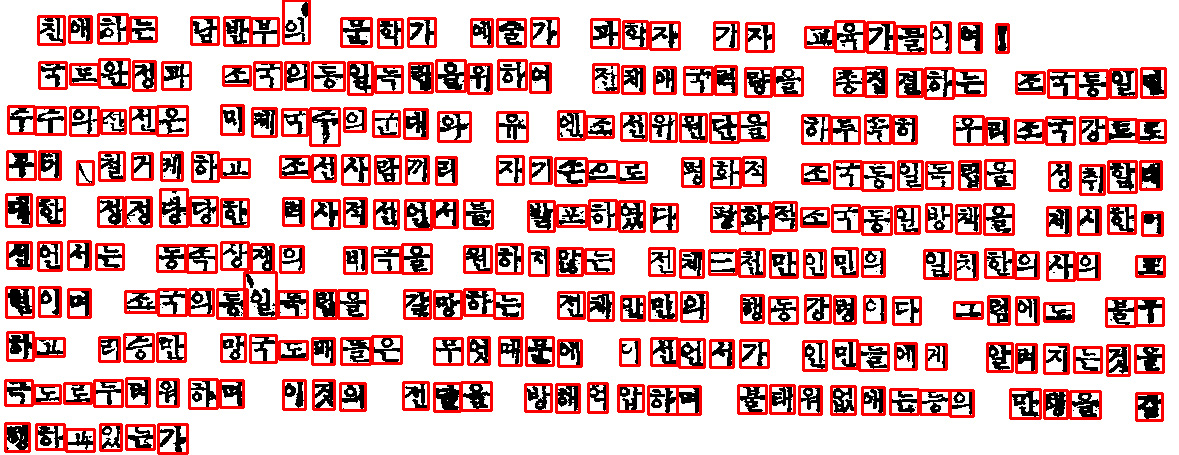
Let’s start by comparing the performances of Tesseract versus Abbyy. We’ll be using Tesseract 3 (the latest version, 4, performs incredibly poorly on Korean) and Finereader 12. For the data, we’ll use the first article printed in 영화 예술 on page 1, an open letter to intellectuals in South Korea (????? ?????? ????????? ??? ????). Rather than process the whole page, we’ll only work on a single paragraph at first, attached below, as this should make the OCR process easier and faster than with a whole page.

Let’s write a quick script to call Tesseract and look at the result:

import pytesseract
from PIL import Image

pytesseract.pytesseract.tesseract_cmd = 'C:\\Program Files (x86)\\Tesseract-OCR\\tesseract'
tessdata_dir_config = '--tessdata-dir "C:\\Program Files (x86)\\Tesseract-OCR\\tessdata"'

img = Image.open('sample.png')

print(pytesseract.image_to_string(img, lang='kor', config=tessdata_dir_config))

???? ????’ ??? ??? ??? ?? ??????? ~ ?

????? ??????????? ??????? ?? ???* ?????
?????? ~`???????? ? ?’??????? ???? ???????
?? ?????? ?????? ????? ??? ??????? ????
?? ?? ??? ??????? ?????“ ?????????? ????
???? ????? ??? ????? ???????? ?????? ?’
??? ???????? ???? ????? ??????? ???? ??
?? ??? ?????? ????? ????? ????? ??????
???????? ??? ??? ?????)? ????????- ??? ?
?????? –

For Abbyy, we’ll have to call the executable, output the result in a text file and then read that into Python:

import subprocess

args = ['sample.png', '/lang', 'Korean', '/out', 'results.txt', '/quit']
p = subprocess.Popen(["C:\Program Files (x86)\ABBYY FineReader 12\FineCmd.exe"] + args)
p.wait()
with open('results.txt', 'r', encoding = 'utf8') as fp:
    x = fp.readlines()

print(x)

???? ???4 ??? ??? ??? ?? ??????!\n???? ? ?????? ???^:? ?? ? ?? ?? ?? ??? ?????4 ?????? , ????????? ????????? ???? ??????? ???????? ?????? ????? ??? ??????? -???? ?? ????? ??? ?.??? ?????& ?????????? ???? ???? ?????? ‘??? ????? ???????? ?????? ? ???: ????????????? ????? ??????/???? ?? ?? ??? ??????- ????? ? ?????????? ?????? ???????? ??? ??? ?????? ???????? ??? ? ???????\t? ,\t? ?:”

While Tesseract’s results are hardly exploitable, Abbyy actually does a very decent job. A lot of the mistakes seem to come from noise in the original scan and look like they could be somewhat improved with a bit of pre and post-processing. While we’re pre-processing the file, we might as well dig a little further and attempt to build our own OCR engine to see if we can improve upon Abbyy’s output. This means following the usual process of OCR preparation with a segmentation of the text in lines and characters. We’ll use Python and the OpenCV library to perform our image manipulations.

To preprocess our document, the first step will be to binarize it in order to separate the content (the text) from its background (the page). To do so, we’ll first turn our image into grayscale then binarize it using Otsu’s method :

import cv2

img = cv2.imread('F:/OCR/sample.png')
gray = cv2.cvtColor(img, cv2.COLOR_BGR2GRAY)
ret2,th2 = cv2.threshold(gray,0,255,cv2.THRESH_BINARY+cv2.THRESH_OTSU)

 

There is still a bit of noise left, but we might be able to get rid of that soon. We will now try to recognize the characters in order to separate them from the meaningless blobs and speckles. To help us do so, we’ll use OpenCV’s contouring function to approximate the shape of each character. We’ll then extract the bounding rectangle for each contour and should see all of our characters neatly delimited by rectangular boxes:

im2, contours, hierarchy = cv2.findContours(th2,cv2.RETR_TREE,cv2.CHAIN_APPROX_SIMPLE)

for contour in contours:
    x, y, width, height = cv2.boundingRect(contour)
    cv2.rectangle(img2,(x,y),(x + width,y + height),(0,0,250),2)

 

The results look promising, we see that a lot of small speckles have been contoured. We could easily get rid of them by specifying some minimum area for our contours, the filter can’t be too large though, as we would risk filtering off actual characters. We also notice that some characters are split into several smaller rectangles bounding their constituting part As contours are made to join continuous points, characters with more space between their constituting parts such as ? or ?, have been separated in different regions. To prevent this problem we can apply morphological transformations to make our black-on-white characters appear thicker and fill the gap between their constituting parts.

Let’s first start with the outliers: we’ll get rid of all the elements within bounding boxes that are either too small or too large to possibly be a character. To ensure that these noisy parts won’t pose a problem at a later stage of processing, we copy the “good” rectangles to an entirely new image. The process is quite straightfrward, as OpenCV uses numpy matrices to store the pictures in memory. We only have to move part of our image’s matrix to a new, blank matrix of the same dimensions:

list_area = []
list_rect = []
new_image = np.zeros(np.shape(th2))
new_image.fill(255)

for contour in contours:
    x, y, width, height = cv2.boundingRect(contour)
    area = width * height
    if area > 50 and area < max_cont_area:
        list_rect.append((x, y, width, height))
        list_area.append(width * height)
        new_image[y : y + height, x: x + width] = th2[y : y + height, x: x + width]

Now we’ll apply our erosion, which will make the black lines of the characters thicker. We will use a narrow and long kernel, this will allow us to blur vertically, keeping the gaps between the characters while minimizing the space within the constituting parts of a character (like the vertical gaps betweens the three bars in ?):

kernel = np.ones((7,7), np.uint8)
img_erode = cv2.erode(new_image, kernel, iterations=1)

Some of the characters on the first line have “lost” their bounding box, which is due to OpenCV’s contouring method (OpenCV contours white areas). To bypass the issue we’ll just have to invert our image. Some characters like ? or ? are still split between two boxes. We could resolve the issue by increasing the width of the erosion kernel, but we would risk losing the otherwise nice separation between characters. A better way to proceed would be to identify the smaller parts and to merge them with their closest neighboring part. By checking that the resulting new part is not significantly bigger than the average box, we can avoid merging boxes that do not belong together and discard those last bits of noise is small, isolated boxes.

We’ll define a function find_outliers to implement the median absolute deviation, which will take a list of integers and a threshold as argument and return a list of booleans. The threshold determines how far away from the median a value would have to be in order to be considered an outlier:

def find_outliers(data, m = 2):
    absdev = abs(data - np.median(data))
    mad = np.median(absdev)
    scaled_dist = absdev / mad if mad else 0
    return scaled_dist > m

We’ll set the threshold a bit high to avoid accidentally getting rid of good characters. Punctuation marks may be affected, but that is hardly an issue. By considering parts that are at least 3 deviations below the median, here is what we get:

outliers = find_outliers(list_area, 3)
median = np.median(list_area)
elements_to_merge = []

for i, rect in enumerate(list_rect):
    x, y, width, height = rect
    if outliers[i] == True and width * height < median:
        elements_to_merge.append(rect)

This looks promising, now all we have to do is try to merge those remaining outliers with their closest neighbor. To find the closest element in each case, we could iterate over all the elements we’ve identified and compare their (x, y) values but that would prove to be quite computing intensive for longer documents. A faster, and not much more complex way to proceed is to take advantage of the scikit-learn library’s built-in functions to build a k-d tree and perform a nearest neighbor search. To do we’ll slightly modify our previous loop. We’ll also store the outliers’ id rather than their rect to make looking them up easier.

For the merging process, we will draw a maximum bounding rectangle parallel to the axes around the elements. If the area of that rectangle is abnormally greater or smaller than the median, we’ll discard the element as noise. The maximum bounding rectangle function will simply take the minimum and maximum top, left, bottom and right coordinates of the subelements to build a rectangle encompassing them:

def minimum_bounding_rectangle(rects):
    list_top = [rect[1] for rect in rects]
    list_left = [rect[0] for rect in rects]
    list_right = [rect[0] + rect[2] for rect in rects]
    list_bottom = [rect[1] + rect[3] for rect in rects]
    min_top = min(list_top)
    min_left = min(list_left)
    max_right = max(list_right)
    max_bottom = max(list_bottom)
    new_rect = (min_left,
                min_top,
                max_right - min_left,
                max_bottom - min_top)
    return new_rect

Taking the nearest neighbor on the simple basis of (x,y) coordinates might seem natural, but risks introducing a bias : when a character like ? gets split into two bits, the x value of the second bit ? might be closer to that of its immediately adjacent character on the right than to the x value of ?, as can be seen on this picture:

 

The (x,y) coordinates for ? will be (0,0.2), for ? it will be approximately (1.8, 0) and for ? (2.1, 0). A better way to proceed would therefore be to compare the coordinates of the elements’ respective centers by computing (x + width / 2) and (y + height / 2). Finally, when filtering the minimum bounding rectangle areas, we can be a little bit more restrictive with respect to heights. The narrow kernel we used for erosion already grouped together elements separated by vertical gaps. The remaining characters that typically get split (?, ?…) therefore tend to be narrower, while height remains constant.

outliers = find_outliers(list_area, 3)
median = np.median(list_area)
elements_to_merge = []
list_x = []
list_y = []
list_heights = []
list_widths = []

for i, rect in enumerate(list_rect):
    x, y, width, height = rect
    list_x.append(x)
    list_y.append(y)
    list_widths.append(width)
    list_heights.append(height)
    if outliers[i] == True and width * height < median:
        elements_to_merge.append(i)

median_width = np.median(list_widths)
median_height = np.median(list_heights)
centers_x = np.add(list_x, list_widths) / 2
centers_y = np.add(list_y, list_heights) / 2
coordinates = list(zip(centers_x, centers_y))
tree = KDTree(coordinates)

merged_elements = []

for element in elements_to_merge:
    dist, ind = tree.query([coordinates[element]], 2)
    mbr = minimum_bounding_rectangle([list_rect[element], list_rect[ind[0][1]]])
    if ((mbr[2] < median_width * 1.5) and
        (mbr[3] < median_height * 1.3)):
        merged_elements.append(mbr)

Now all we have to do is combine this new list of merged elements with the previous list of characters that were already properly segmented:

    
median_width = np.median(list_widths)
median_height = np.median(list_heights)
centers_x = np.add(list_x, list_widths) / 2
centers_y = np.add(list_y, list_heights) / 2
coordinates = list(zip(centers_x, centers_y))
tree = KDTree(coordinates)

merged_elements = []
clean_list = list(set(list_rect))

for element in elements_to_merge:
    dist, ind = tree.query([coordinates[element]], 2)
    mbr = minimum_bounding_rectangle([list_rect[element], list_rect[ind[0][1]]])
    try:
        clean_list.pop(clean_list.index(list_rect[element]))
    except:
        pass
    if ((mbr[2] < median_width * 1.5) and
        (mbr[3] < median_height * 1.3)):
        try:
            clean_list.pop(clean_list.index(list_rect[ind[0][1]]))
        except:
            pass
        merged_elements.append(mbr)
        clean_list.append(mbr)

[/source]

<a href="http://digitalnk.com/blog/wp-content/uploads/2017/09/somelastbugs.jpg" rel="attachment wp-att-86"><img class="wp-image-86 size-large" src="http://digitalnk.com/blog/wp-content/uploads/2017/09/somelastbugs-1024x395.jpg" alt="" width="640" height="247" /></a> Almost there

<a href="http://digitalnk.com/blog/wp-content/uploads/2017/09/somelastbugs.jpg" rel="attachment wp-att-86"></a>

The merge process left some overlapping rectangles, maybe a result of smaller areas merging together rather than with their larger neighbor. Going back to the previous phase and adding code to handle these cases would prove unnecessarily complicated, when we can simply go over our areas again and check for overlaps using the same nearest neighbor algorithm. Once the last overlapping rectangles are merged, we can copy the content within the segmented coordinates on the earlier binarized picture and copy them to a new, clean image, which will give us our result:



clean_list = list(set(clean_list))

coordinates = [((l[0] + l[2]) / 2, (l[1] + l[3])/  2) for l in clean_list]
tree = KDTree(coordinates)

final_list = list(clean_list)
for element in merged_elements:
    dist, ind = tree.query([((element[0] + element[2]) / 2, (element[1] + element[3]) / 2)], 2)
    nearest_neighbor = ind[0][1]

    if (element[0] >= clean_list[nearest_neighbor][0] and
        element[1] >= clean_list[nearest_neighbor][1] and
        element[0] + element[2] <= clean_list[nearest_neighbor][0] + clean_list[nearest_neighbor][2] and
        element[1] + element[3] <= clean_list[nearest_neighbor][1] + clean_list[nearest_neighbor][3] and
        clean_list[nearest_neighbor] != element):
        try:
            final_list.pop(final_list.index(element))
        except:
            pass


clean_image = np.zeros(np.shape(th2), dtype=np.uint8)
clean_image.fill(255)
     
for rect in final_list:
    clean_image[rect[1] : rect[1] + rect[3], rect[0]: rect[0] + rect[2]] = new_image[rect[1] : rect[1] + rect[3], rect[0]: rect[0] + rect[2]]

There’s still a bit of noise here and there, but most of it we should be able to deal with it afterwards when we work on line segmentation. For now let’s see how our current script works with more text:

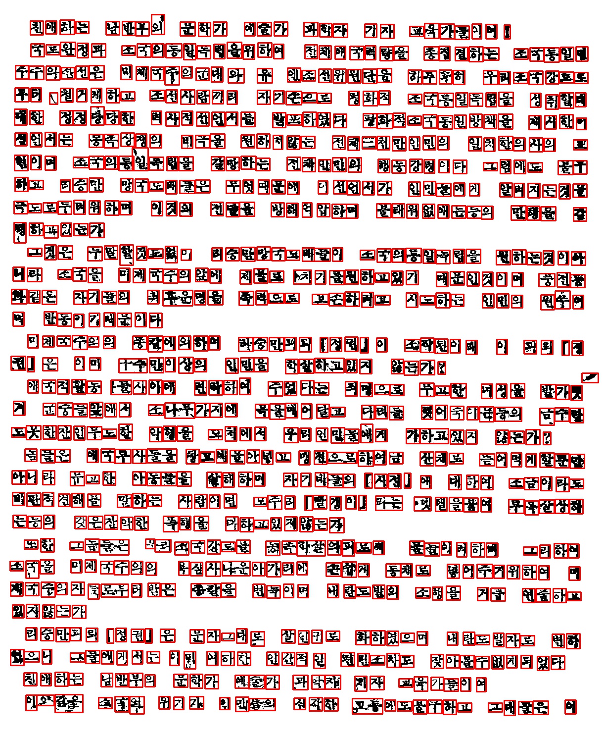
A few adjacent characters are still enclosed together here and there, but again, we can deal with this later when parsing the lines. We’ve coded the algorithm to work on pictures of homogeneously formatted text, but let’s see how it performs on the full page, with the title in a larger font size and more noise on the page’s edges:

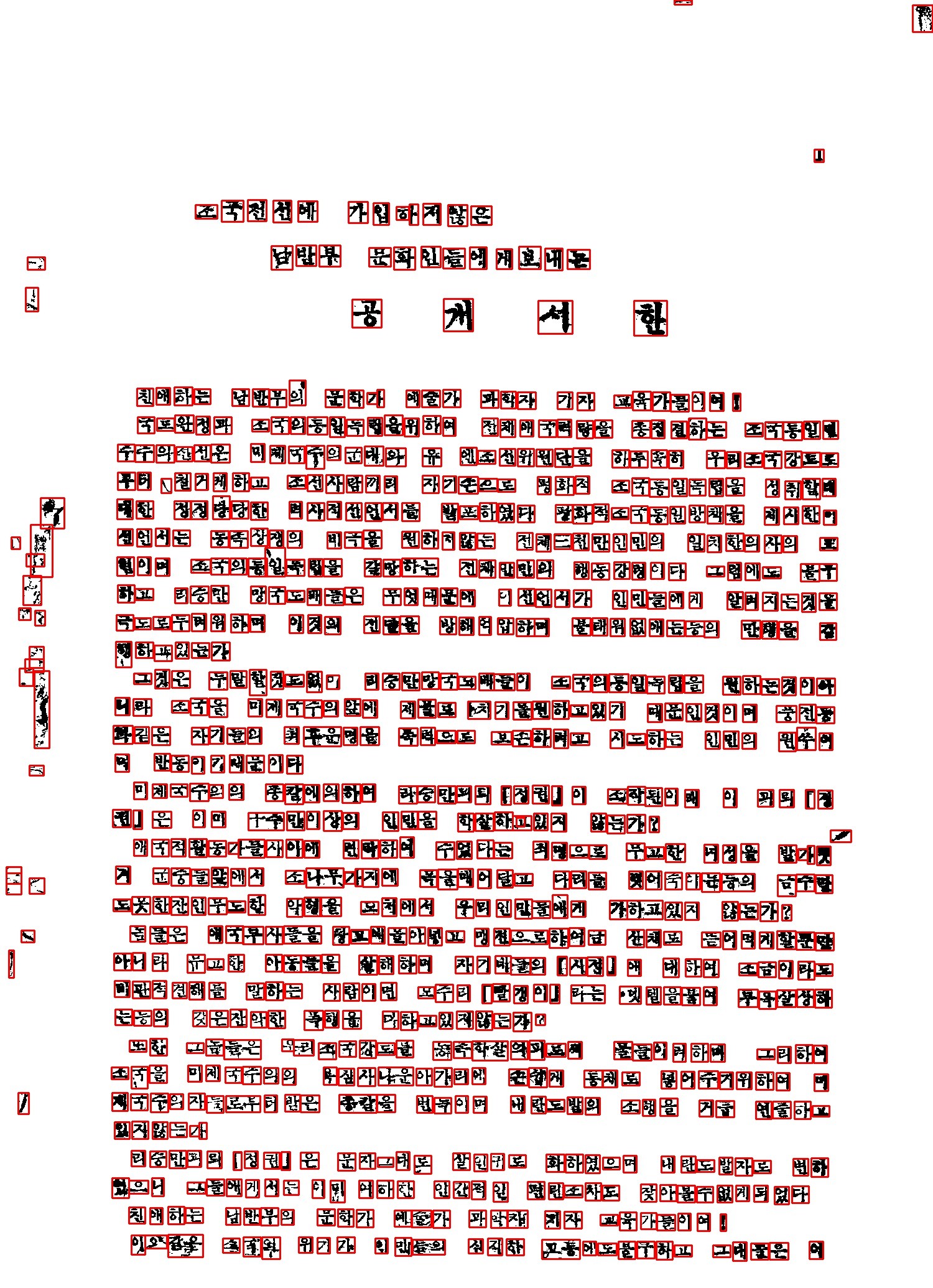
Not bad. We see that the article’s title was properly segmented even though the font size is fairly different. Certain characters like ? or ? are still split in two, which is unfortunate. However, this might simply be due to the fact that we are feeding the algorithm a “raw” document : the different font size for the title and the noise on the edges introduce more variation and are probably skewing our median-based calculations, so that the smaller rectangles of these split characters are no longer detected as outliers. So we can expect these problems to be largely gone once we apply more pre-processing to the documents, to remove unnecessary margins and separate the title and the body of the article.

Full code is on Github.